You as a manufacturer (or entrepreneur or craft business owner or whatever you like to call yourself) have probably heard of Lean Manufacturing and wondered if it’s an idea that has value for your business.
And if you’re a regular here at Zattatat, you know from reading some of our recent articles that Lean Manufacturing is a cluster of ideologies that strive to minimize waste and inefficiency in a manufacturing operation, with the goal of producing high quality items for a low price and on a fast schedule. (The Toyota Production System is an example of a specific Lean Manufacturing model.)
But we can’t really cover Lean Manufacturing without also talking about the closely related subject of…
Six Sigma
Yes, if you’re in the world of making/producing/manufacturing you’ve probably heard of Six Sigma at least in passing.
Invented by Motorola engineer Bill Smith in the 1980s, Six Sigma is a system for improving manufacturing quality. Since it’s not a system directly focused on reducing waste or improving efficiency, it’s not technically considered a Lean Manufacturing framework.
But Six Sigma does dovetail well with the Lean Manufacturing subgoal of delivering high-quality products, and with the broader concept of improving operations/manufacturing performance.
So what exactly is Six Sigma?
Glad you asked ;
If you’re familiar with the mathematical subject of statistics, you know about Normal Distributions, also called Bell Curves.

The horizontal dimension of the graph (x-axis) is any parameter that’s important to quality control on your manufacturing line.
For example, Gary makes cookies.

So Gary’s parameter or interest, or his x-axis on the graph, is the thickness of the cookies in millimeters.

And the height on the graph is how common an occurrence is.
So if we look at that same graph again, remembering that the left side is the very thin cookies and the right side is the very thick cookies…
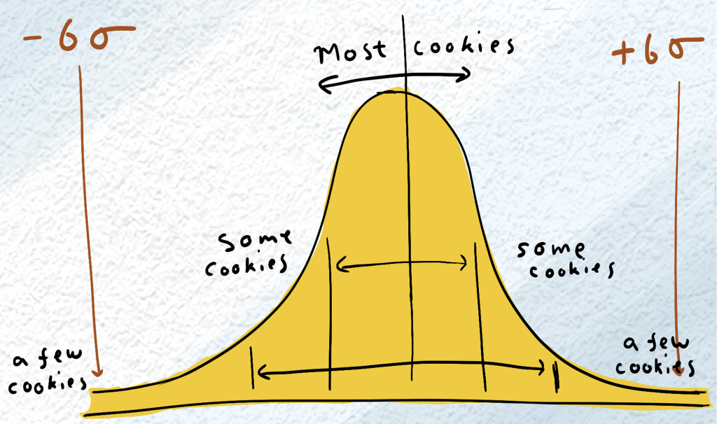
A graph that looks roughly like this is called a…
Normal Distribution.
Not everything you’ll ever try to model with statistics will give a graph of this shape. But yes, this general pattern is so common across so many things in the natural sciences, social sciences, and applied sciences (like engineering and manufacturing!) that it’s simply called the “Normal” distribution. In our Normal Distribution, most cookies are of close-to-average thickness; some are a little bit thick or a little bit thin; and a few are very thick or very thin.
So why is it called Six Sigma?
The Greek character Sigma is used in the field of statistics to represent the concept of Standard Deviation. In the graph above, you’ll notice that the labels of -6 Sigma +6 Sigma (meaning – or + 6 standard deviations from the average cookie thickness) are very rare occurrences. Hardly any cookies are that thick or that thin.
Now, if you know what standard deviation is, great!
If not, here’s a simple way to understand it, again using our cookie example:
There’s an average thickness to the cookies. Let’s say it’s 1 centimeter.
But each individual cookie’s thickness is NOT exactly 1 centimeter. One cookie is 0.8cm, one is 1.5cm, etc.
Standard deviation is (essentially)*, the average difference between the thickness of any random cookie and that of the average cookie.
Huh?
Fine, that was confusing. But I promise it’s not that complicated!
Our average cookie was 1cm. Cookie #1 was 0.8cm, so its difference from the average was 0.2cm. Cookie #2 was 1.5cm so its difference from the average was 0.5cm. If cookie #3 is 0.6cm, its difference from the average is…
(You said 0.4cm, right?)
So if we take the average of the difference from the average from that sample*, we get (0.2cm+1.5cm+0.4cm)/3 = 0.77cm. The average difference between any random cookie and the average cookie is 0.77cm in our example. So 0.77cm is our standard deviation, or our Sigma.
And this is relevant to quality control because (to use our cookie example again), we want to make our process consistent enough that our upper and lower tolerance limits (which we set based on our own criteria, like customer satisfaction or fitting into the cookie box) are six standard deviations (Six Sigmas) away from our average. In other words, we’re having to throw out very few cookies!
Ok, maybe that was a bad example because with cookies…

But you get the point 🙂
Weekly Challenge:
Look through your own business and see if there are areas where this Six Sigma concept could help with your quality control! And come back next time to see exactly how Lean Manufacturing and Six Sigma are now being used together in modern manufacturing theory.
*As you’ll know if you’ve taken a formal statistics class, this is not exactly how standard deviation is calculated. But it’s a simplified formula that explains the concept well enough for our purposes 🙂